
ML 101 - How does the k-Means algorithm work?


This is article #7 in the “ML 101” series, the purpose of which is to discuss the fundamental concepts of Machine Learning. I want to ensure that all the concepts I might use in the future are clearly defined and explained. One of the most significant issues with the adoption of Machine Learning into the field of finance is the concept of a “black box.” There’s a lot of ambiguity about what happens behind the scenes in many of these models, so I am hoping that, in taking a deep-dive into the theory, we can help dispel some worries we might have about trusting these models.
Unsupervised learning, also known as pattern recognition, is a method that attempts to find intrinsic patterns in a dataset without an explicit direction or end point in the form of labels. In colloquial English, in a supervised learning problem, we might tell a model to “find the optimal general path from a set of inputs to the exact desired outputs (in classification) or as close as possible to the outputs (in regression)”. In an unsupervised learning problem however, with the absence of our definite output, we will tell a model to “uncover some hidden relationships in the data that might not be obvious at first glance and use this to create distinctions between different groups”.
One of the benefits of unsupervised learning is that it helps us discover latent variables. Latent variables are variables that are not explicitly obvious in our dataset. They are hidden in our dataset and are generally inferred or produced by combining more than one feature in some mathematical way. Without any knowledge of what the intended target is to influence the model, it looks at the dataset in a more abstract way, finding relationships that may be more robust than those found in a supervised learning problem.
k-Means
K-Means Clustering will take a set of variables and find K clusters, or groups. These clusters are intended to be distinct, but for the data points within them to be similar. The idea is that we are able to partition our dataset into K groups, which might tell us a little bit more about their implicit characteristics. Each cluster is defined entirely by its centre, or mean value, mu_k.
This is a good method to employ during the exploratory data analysis phase of your machine learning workflow because it gives us the opportunity to take a blank, fresh dataset and allow a model to give us some pointers as to where we might find interesting relationships.
The mathematical notation of the model and its outputs are shown below
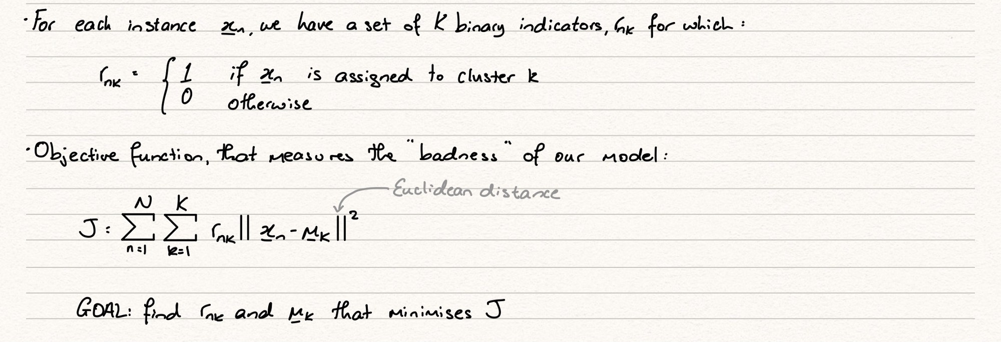
K-Means begins by plotting all the data points in an n-dimensional space, where n is the number of feature variables that we have. For example, 3 features will be plotted on a 3D graph, 4 features will be plotted on a 4 dimensional space and so on… With this visualisation, the model will attempt to assign points in the data, our means, in the middle of which there are obvious groupings of similar data points. Iteratively, the model will continue to improve the value of the mean, using a cost function that minimises within cluster distance and maximises between cluster difference.
The pseudo code for the K-Means algorithm is as follows:
1. Initialise mu_k randomly
2. Minimise J with respect to r_nk, without changing mu_k
3. Minimise J with respect to mu_k, without changing r_nk
4. Repeat until the two minimisations converge
Consider that we have intialised our mean value. We will now plot it on our graph with our data and assign a class to each instance depending on the mean value it is closest to. This is how we will minimise in step 2. The concept is that we will then move to step 3 and attempt to find a better mean and then return back to step 2 to see how this new mean changes the r_nk value. As step 4 tells us, we continue this sequence until we find convergence.
To show the notation of step 2:
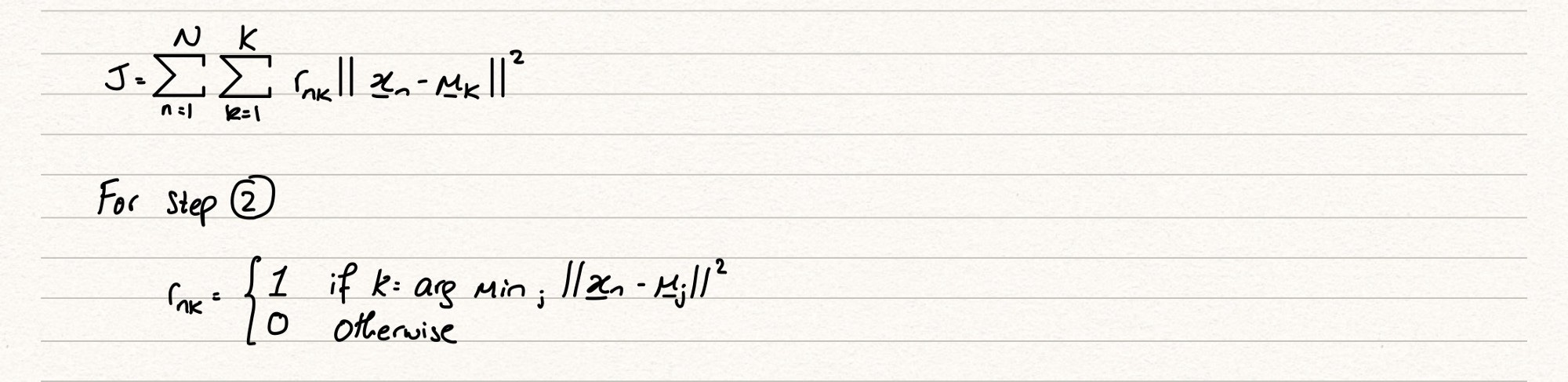
In the second part of the above image, we are saying that we will assign the r_nk to be 1 if the j value, determined by which cluster mean we are measuring, returns the lowest distance i.e. is the cluster that we will assign this instance x_n to.
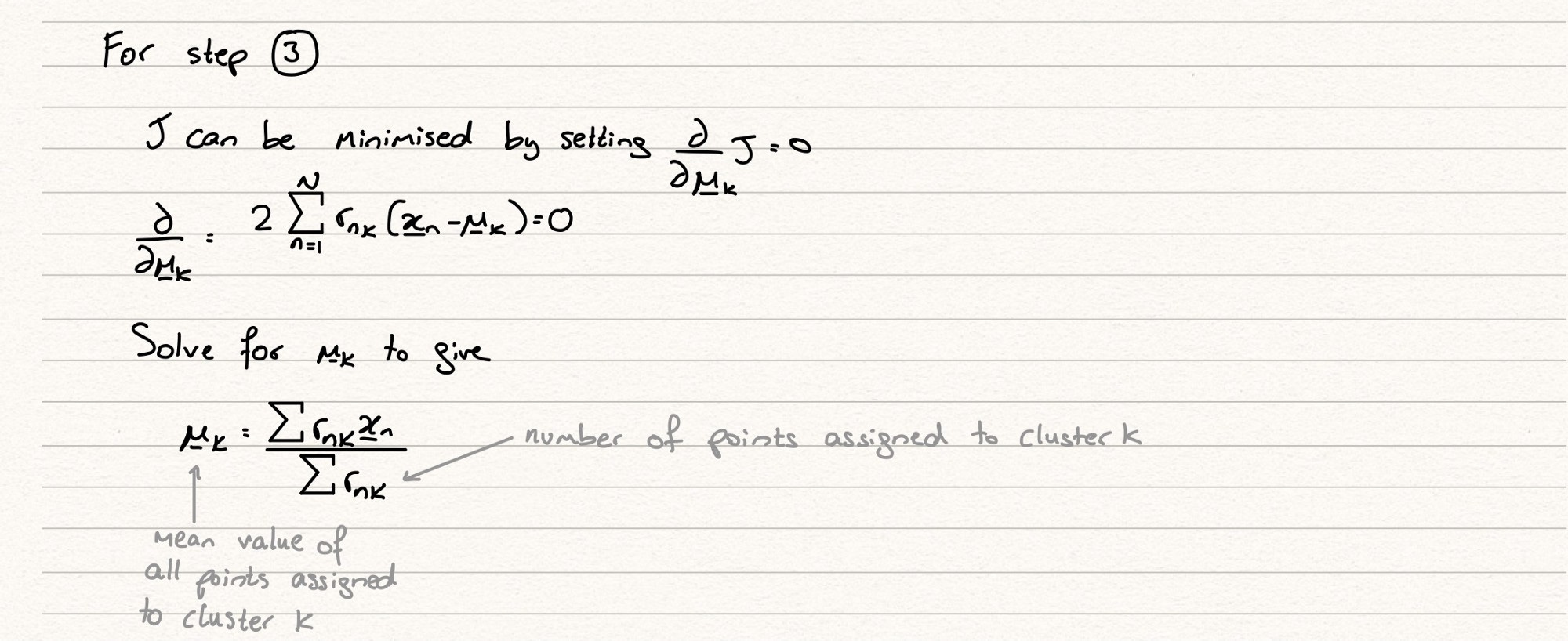
Step 3 involves us trying to minimise the mean of each of our clusters. This is a quadratic function, as we can see from the equation. We can therefore minimise J by differentiating, setting the solution equal to 0 and solving.
The diagram below shows the evolution of a typical k-means clustering algorithm. We can see here how our iterative algorithm will converge towards an optimal solution for 2 distinct clusters.

Some features of K-Means that we should be aware of are as follows:
We are guaranteed convergence because of the differentiability of the optimisation algorithm, but we run into the issue of reaching a local minima instead of the global minima and because of this…
…we are largely dependent on the initial mean values into order to find the global minima
It is difficult to define the optimal number of clusters, so this may take some fine tuning and iteration
K-Means is an expensive algorithm, as each iteration requires K*N distance comparisons
Every instance is assigned to one cluster and one cluster only, which may be problematic if we have some instances that might belong to more than one cluster
The distance calculations are sensitive to outliers
The Elbow Method
We can address one of these points in more detail. How do we select the optimal number of clusters, K? The elbow method is how we do this. Typically, as we increase the clusters, we will expect the cost function, J, to fall because every time we add another mean it reduces the distance to some instances. There is, however, a trade off here, in that as we continue to add more cluster means, the higher the chance of overfitting our data. This is understandable, because we are continually increasing the number of clusters in order to get a better fit on our training data, without paying any attention to how this model might operate on our test data. It’s always key to remember that we want a solution that can generalise and therefore not one that is too fixed to our training data but one that can adapt to different unseen inputs and still give us good results.
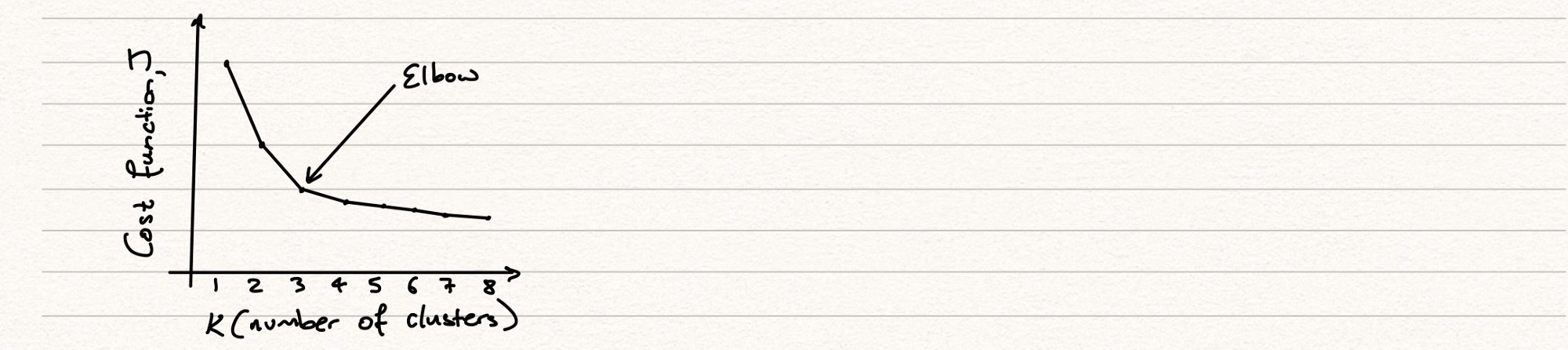
The elbow is the point after which we begin to see a diminishing rate of return. The benefit to us adding another cluster is not proportional to the added complexity of our model. We would find this elbow by running through a series of simulations with different numbers of clusters, plotting their cost functions and observing the graph, which we would expect to look similar to the one above.