

Algorithmic Trading Models - Moving Averages
Algorithmic Trading Models - Moving Averages

In the second article of this series, we will continue to summarise a collection of commonly used technical analysis trading models that will steadily increase in mathematical and computational complexity. Typically, these models are likely to be most effective around fluctuating or periodic instruments, such as forex pairs or commodities, which is what I have backtested them on. The aim behind each of these models is that they should be objective and systematic i.e. we should be able to translate them into a trading bot that will check some conditions at the start of each time period and make a decision if a buy or sell order should be posted or whether an already open trade should be closed.
Please note that not all of these trading models are successful. In fact, a large number of them were unsuccessful. This summaries series has the sole objective of describing the theory behind different types of trading models and is not financial advice as to how you should trade. If you do take some inspiration from these articles, however, and do decide to build a trading bot of your own, make sure that you properly backtest your strategies, on both in and out of sample data and also in dummy accounts with live data. I will cover these definitions and my testing strategies in a later article.
When taking an initial foray into algorithmic trading, or any form of building trading models, a moving average model is one of the easiest to both understand and implement. From my initial research, moving average models can be split into 3 types, which we will summarise below. Before we do that however, we do need to define exactly what a moving average is and the different types of moving averages.
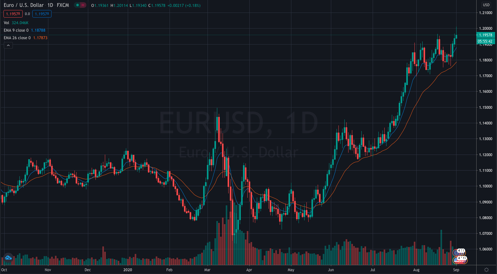
Simply put, a moving average calculates a series of averages of a time series, with the aim of removing noise and showing us the trend of the prices. There are 3 commonly used moving average types that we will detail.
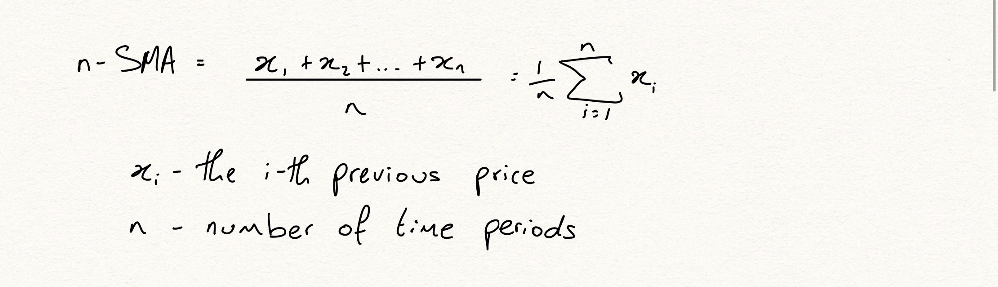
A simple moving average calculates each value as the mean of the previous n values. We describe this as an n period SMA, or n-SMA.
The exponential and weighted moving averages are similar in their calculated in that they both include applying weights to each data point. They differ however, in the way that these weights are calculated, namely exponentially and linearly. The weights in our EMA are assigned such that the most recent data point has the greatest influence over the EMA value in an exponential manner, whilst the WMA weights rise at a uniform rate (linearly). The one requirement for both types of moving averages is that their weights must sum to 1.
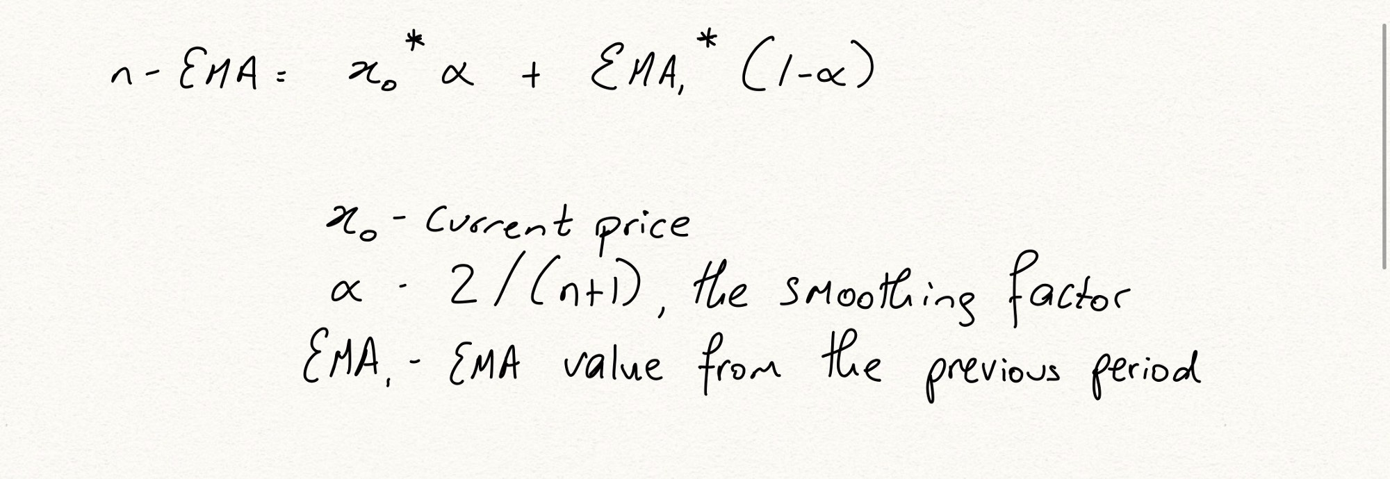
The EMA calculates the weight for the most recent data point using a smoothing factor, which we will call alpha. The smoothing factor is calculated by taking 2 / (1 + time_period). For a 10 period EMA, this will be 2/(10+1) = 0.1818, for a 20 period EMA this value will be 0.0952. This value, along with the value for the previous time period’s EMA will be fed into the following formula to calculate the current EMA.
As you can see, if we were to take the 10 period EMA as an example, the most recent data point is assigned roughly an 18% influence over the EMA value, whilst the previous 10 data points, represented by the previous EMA, are assigned a 72% influence.

The advantage of the SMA is that is provides us with a smoother line. For this reason, it is more commonly used by traders on longer timeframes, daily and weekly charts. The SMA is less likely to react to whipsaws, giving us a better idea for the overall market trend. The disadvantage, is that the lag of the SMA means that we will miss out on picking up trend changes quickly. This is where the WMA and EMA attempt to adjust for this issue. The weightage system allows these two moving averages to react more to recent price changes, allowing us to identify when trends are shifting closer to the exact point that the shift happened.
It is worth noting at this point that there are many more types of moving averages we could use for our analysis and with a powerful machine, we could easily iteratively test all these strategies on many different moving average types to find the most effective.
Strategies
So we have 3 models that we can use that incorporate moving averages. There are of course others, but we are looking for models that can be quick easily incorporated into a trading bot.
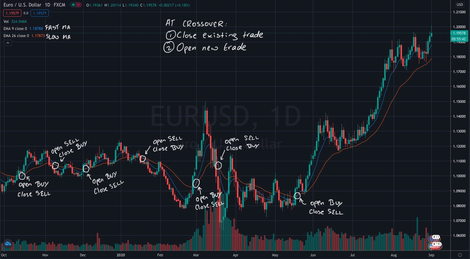
Moving Average Crossover Model
Trend Following Model
Dynamic Support and Resistance Model
The first is a very simple moving average crossover model. The theory behind this is that, when observing the values of a slower and faster moving average, the point at which they crossover indicates a change in the trend. To translate this into systematic rules, we post a buy order as soon as the fast moving average crosses above the slow moving average and we post a sell order as soon as the fast moving average crosses below the slow moving average. We then set our stops as the point in which the next crossover is observed i.e. a signal reverse, or a fixed value, such as a specific number of pips away from the open price or a multiple of the average true range of the previous x periods.
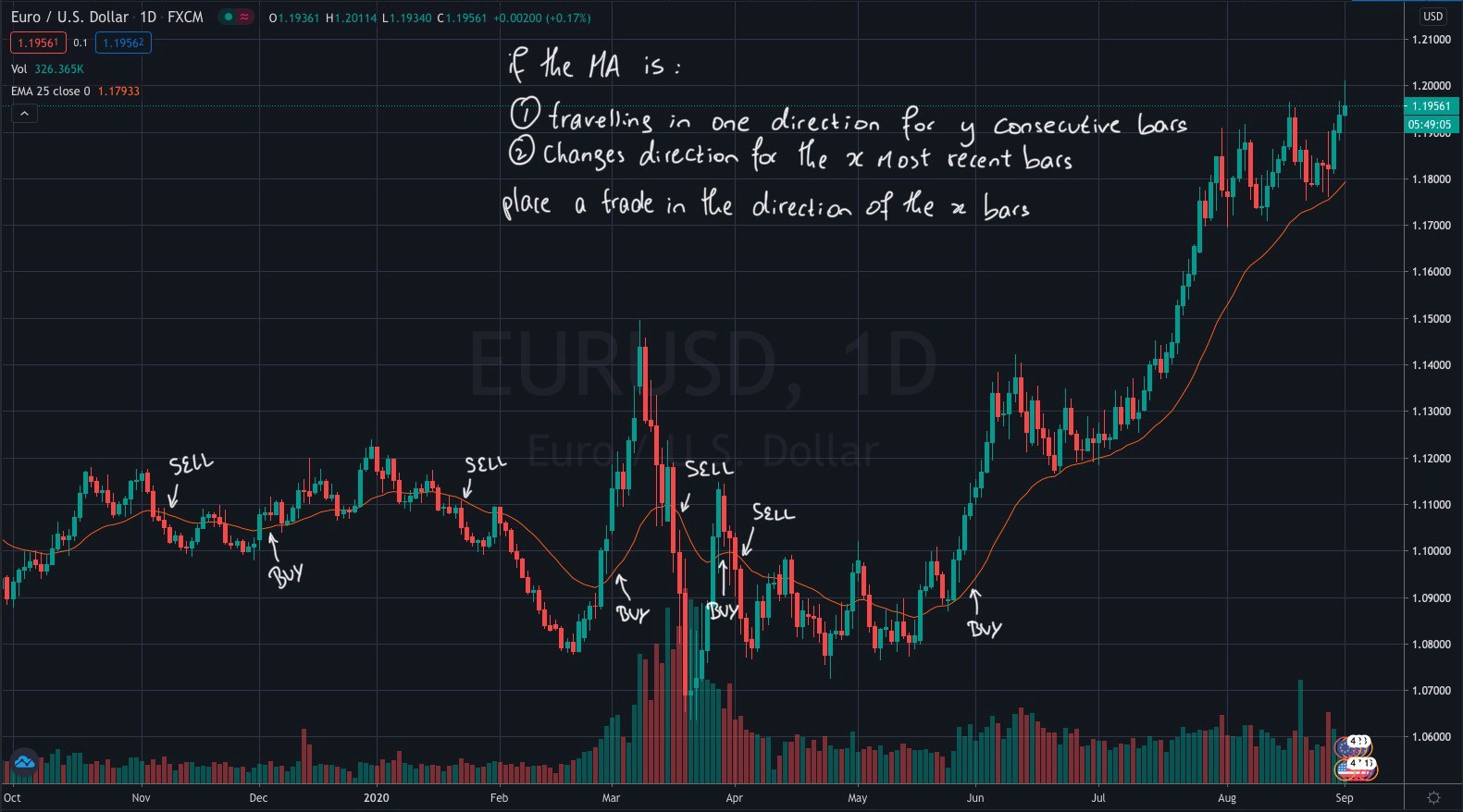
The second model is a trend following strategy. We only require one moving average here, for which we observe the initial direction. As soon as we see a reverse in direction for x consecutive bars, we place a trade in the new direction. The theory here is that we have identified a new trend and aim to enter the market as close to the start of the trend as we can. The standard stops, as mentioned above, are used.
The final moving average model that we will consider is a support and resistance strategy. In many situations, we may observe that a moving average acts as a dynamic support and resistance. In an uptrend, we may see many pullbacks in the market that drop down to a moving average, before bouncing off again, as though the moving average is the support level. Similar behaviour is observed in a downtrend, but in that case, the moving average is a resistance level. What we might aim to do is enter a trade in the initial direction, on a pullback. If the price drops down to touch the moving average, we will place a buy order. If the price rises to touch the moving average, we will place a sell order. The advantage of this strategy is that, if the moving average is acting as a dynamic support or resistance, we will have found as close to an optimal entry as we can hope to achieve, since the price will be expected to bounce straight away and continue the long term trend. The standard stops are to be applied.
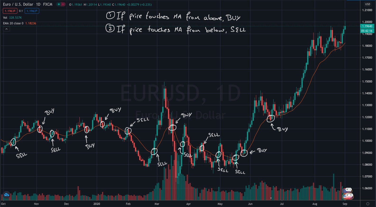
As you can see, particularly with the moving average bounce strategy, there is a lot of scope for optimisation and adding protocols to avoid entering a breakout. There are areas of this chart where the 20 period EMA seems to act as a perfect support level, but in other scenarios our price breaks through this line and continues to move in its original direction.