

ML 101 - Decision Trees: The Maths, The Theory, The Benefits
ML 101 - Decision Trees: The Maths, The Theory, The Benefits


Just before we begin this article, I wanted to let you know that you can also find Algo-Fin now on Twitter. We recently launched an account where we’re looking to post end-of-week forex summaries and comments on important news releases. You can click on the tweet below to check out our account and give it a follow!

This is article #4 in the “ML 101” series, the purpose of which is to discuss the fundamental concepts of Machine Learning. I want to ensure that all the concepts I might use in the future are clearly defined and explained. One of the most significant issues with the adoption of Machine Learning into the field of finance is the concept of a “black box.” There’s a lot of ambiguity about what happens behind the scenes in many of these models, so I am hoping that, in taking a deep-dive into the theory, we can help dispel some worries we might have about trusting these models.
Introduction
Most common Machine Learning methods, such as classic Linear Regressions, Classifications, K-Nearest Neighbors, use a metric cost function to evaluate performance. As an example, we use the Euclidean distance in a kNN algorithm to find the closest k data points to our unseen one and use the classes of these observed points to assign a value.
There are some datasets or problem questions that do not align perfectly with this method of analysis. Classifying fruit based on its description does not benefit from a calculation of euclidean distances or l1 distances at any point in the process, so we need an alternative method that can attack these specific problems.
What we might notice about problems that do not lend themselves to distance calculations is that they might benefit from a model that aims to “categorise” them better. Essentially, a model that is less mathematically intense (on the surface) and aims to find common data points by splitting a dataset into progressively smaller and smaller groups at every iteration. The idea is that when we reach the end of our model, we will have a series of groups that can be uniquely identifiable as belonging to a specific class.
This is essentially the process of a Decision Tree. Decision Trees apply a sequence of decisions or rules that often depend on a single variable at a time. These trees partition our input in regions, refining the level of detail at each iteration/level until we reach the end of our tree, also called leaf node, which provides the final predicted label.
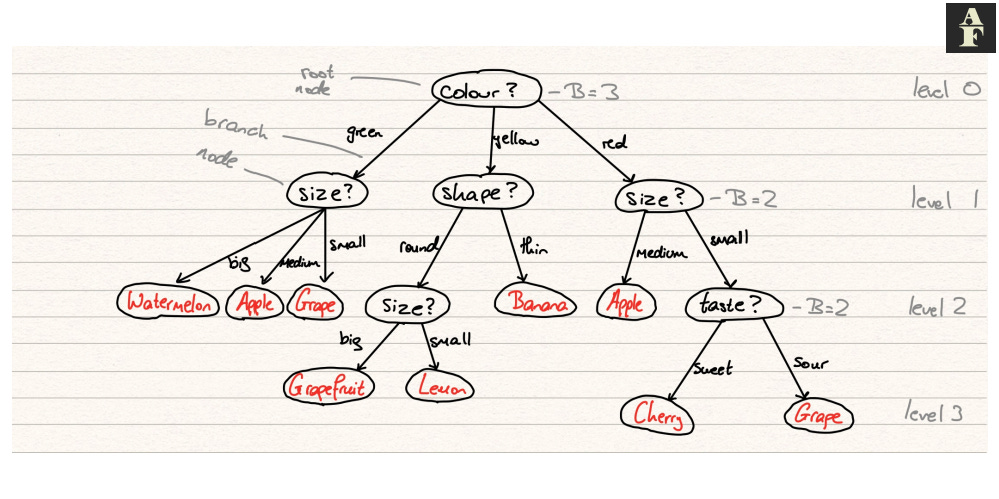
Components of a Tree
A decision tree has the following components:
Node — a point in the tree between two branches, in which a rule is declared
Root Node — the first node in the tree
Branches — arrow connecting one node to another, the direction to travel depending on how the datapoint relates to the rule in the original node
Leaf node — a final node in the tree, a point at which a label is assigned to the data point
Level — a number assigned to each set of nodes, starting from 0 that denote how many levels those nodes are from the root
Branching factor — the branching factor B at level l is equal to the number of branches is has to nodes at level l+1
So how does an instance pass through a decision tree? We begin at the root node. This node will have some declaration e.g. “the animal has more than two feet” or in mathematical notation, passing in an array in which the first value dictates the number of feet of said animal, we have x[0] > 2. We evaluate our instance with respect to this function and decide which branch we must now go down to reach the next level. It’s important to note that the branch decisions must be mutually exclusive, meaning that there cannot be any uncertainty as to which direction the input will move to (it must be purely objective). The node that we have moved to is now considered the root node of this new subtree and we start the process again. This continues iteratively until we reach a leaf node and assign the associated class to our instance.
Tree classification is considered to be extremely interpretable and very quick to execute, since simple decisions are being made at every stage and an entire tree does not need to be traversed in order to find the correct class. Our trees will also calculate, through training, what the most influential feature variables are, so we may not even need to assess all feature variables in order to make a decision on the class.
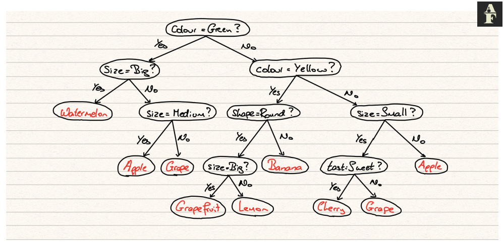
Binary Trees
The simplest type of tree is a binary tree. A binary tree contains a maximum branching factor of 2 at every level. Every parent node can therefore have a maximum of 2 child nodes. In most cases these may be Yes/No decisions.
Every tree with a branching factor greater than two can be recomposed into an equivalent binary tree. This is sometimes a useful feature due to simplicity. In most programming languages, you can specify whether you want to restrict any decision tree model to just a binary tree structure.

The Maths
The maths in decision trees occurs in the learning process. We initially start with a dataset D = {X, y} from which we need to find a tree structure and decision rules at each node. Each node will split out dataset into two or more disjoint subsets D_(l,i)*, where l is the layer number and i denotes each individual subset. If all our labels in this subset are of the same class, the subset is said to be pure and this node will be declared a leaf node and this section of the tree has reached termination. If this is not the case, the splitting criteria will continue.
In some, more complicated datasets, to get to a stage in which every leaf node is pure may require extremely deep decision trees that will lead to overfitting of the dataset. Due to this, we often stop before we arrive at pure nodes and instead have to develop some more sophisticated termination strategies in which the nodes may be impure but the error is accounted for and measured.
Trees are called monothetic if one attribute is considered at each node and are called polythetic otherwise. We generally prefer simpler trees because these are easier to interpret and execute. In most programming languages it is possible to restrict a decision tree to create either monothetic or polythetic trees, but it’s almost always advisable to try the former first and only increase in complexity if absolutely required. To create these trees , we minimise a measure that we call impurity.
Impurity Measures
Entropy impurity or information impurity is calculated using the following formula:
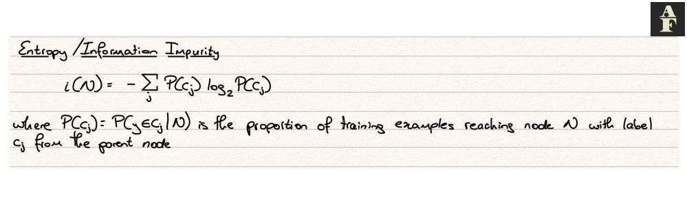
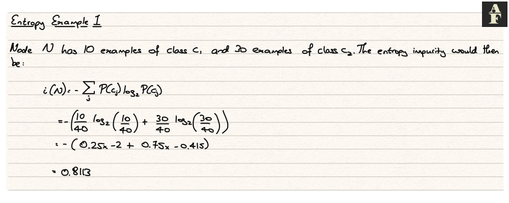
This formula essentially tells us the level of predictability at each node in our tree. Ultimately we want our notes to be predictable and we achieve this by ensuring there are a large majority of a specific class in a node. To display the difference between different levels of predictability and to highlight the effect this has on our impurity measure, I have included some examples below.
Since we want our information impurity value to be as close to 0 as possible, we have a minimisation problem. Our model will run through each variable and its possible values to find the statement (such as x[0] > 2 or x[3] = 1) that will lead to the lowest impurity values for the child nodes.
Stopping Criterion
We know that we cannot always expect our tress to form perfectly pure leaf nodes and because of this, we have to establish some form of stopping criterion. We can do this in a few different ways.
For the validation set method, we spit our training data into a training set and a validation set. Typical splits are 66%-34% or 70%-30%, but this is at the discretion of the user. Our model will continue to split our subsets, creating more branches and nodes at every level and whilst it does this, it measures the error on the validation set. As long as the error on the validation set continues to fall, we continue to split our subsets. When the error stops falling, we stop the generation of new levels to our decision tree and this is our final model.
Pruning is a method used to simplify our tree post training. We start by running our decision tree model and training a full tree, without any stopping criterion. After this we measure the impurity at each node. We then run through each pairs of leaf nodes and eliminate those that do not cost us a high impurity penalty, essentially removing a set of branches from our tree. We continue to do this either a predetermined number of times, or as many times that our impurity penalty is below a certain threshold.
Regression Trees
Technically, decision trees can be used in regression analysis. In this case, the leaf nodes become continuous values. The label of a leaf node is the mean of the data points that are assigned to that node.
Typically, decision trees aren’t used in regression. Their structured nature, particularly the way in which they make hard decisions at each stage lend themselves far more to a classification problem. More often than not, other models more applicable to regression analysis will land up performing better than decision trees.
*D_(l,i) represents D_subscript_(l,i)